Revision as of 23:29, 2 January 2010

Biomolecular Graphics: In Principle and in Practice

Overview, general notes

Figures

This section illustrates the figure-creation process, from initial conception → final multi-panel figure ready for publication. Organized as various "case studies" that are representative of the tasks typically faced by structural or computational biologists, this section provides several step-by-step examples. These examples are entirely self-contained, and the materials include everything from (i) raw, starting data (e.g., PDB files) to (ii) actual, working PyMOL or Python scripts and (iii) final output image files.

Case 1: Overall fold / domain level (≥ novice/intermediate)

Stereo view of a protein fold

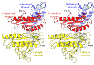
Illustration of the overall fold of carbonic anhydrase, CsoS3, from Halothiobacillus neapolitanus.(PDB ID 2G13). The three domains that compose this enzyme are distinguished by coloring each domain separately (blue, yellow, red). The orientation was chosen to feature the location of the active site (outlined by side chains and zinc ion), and to show the two-fold symmetry relationship between the active domain (yellow) and homologous but defunct domain (red). SSEs are labeled directly on the individual SSEs. Domain labels are colored to correspond to the domains they are labeling. Labels in the active site are given an “outer glow” to make them legible in a region of the figure that is dense in detail. Depth is conveyed by use of fog, veiling less important structural features in the back of the enzyme.

Ingredients for this figure:

1) Download Coordinates

2) Download Pymol script

3) Run Pymol script

#BEGIN PYMOL SCRIPT for Overall Fold -left half of stereo image

#   antialias =1 smooths jagged edges, 0 turns it off
set antialias = 1

# Larger values of ambient make the image brighter
set ambient=0.3

# Larger values of direct eliminates shadows
set direct=1.0
set ribbon_radius =0.2

# cartoon_highlight_color will give a separate color to edges of secondary structural elements.
set cartoon_highlight_color =grey50

# ray_trace_mode=1 makes a black outline around the secondary structural elements
set ray_trace_mode=1

#   stick_radius -adjust thickness of atomic bonds
set stick_radius = 0.2

#   mesh_radius -to adjust thickness of electron density contours
set mesh_radius = 0.02

#   bg_color --set the background color
bg_color white

#   load pdb file and give it an object name
load csos3_18o_nobreak.pdb, csos3

#   hide nonbonded atoms (i.e. waters)
hide nonbonded

#   show cartoon ribbons
show cartoon

#   Hide the default line representation of atomic bonds
hide lines

#   Use standard helix, strand, and loop representations
#   other possibilities: cartoon loop, cartoon rect,
#   cartoon oval, and cartoon tube
set cartoon_tube_radius, 0.2

#   If you dont have secondary structure assignments
#   in the PDB header then get secondary structure assignments 
#   from dssp  http://swift.cmbi.kun.nl/gv/dssp/
#   Then convert assignments into a PDB header
#   http://structure.usc.edu/dssp2pdb/
#   If you want to define secondary structure manually, 
#   Use the following syntax 'S'=strand 'H'=helix
#   alter B/753:758/, ss='S'


#   Make fancy helices with ridge on the edges like
#   molscript does
#   1 is on.  0 is off.
set cartoon_fancy_helices=1
set cartoon_cylindrical_helices=0

#   Make the strands flat=1 or pass through CA positions=0
#   Set to 0 when showing side chains from a strand
set cartoon_flat_sheets = 1.0

#   Draw the loops smooth=1 or pass through CA positions=0
#   Set to 0 when showing side chains from a loop
set cartoon_smooth_loops = 0

#   Set the color of the residues
#   to find the names of the colors available
#   click on the rainbow colored square in the
#   upper right corner of the graphics window
#   Here I make some customized colors as mixtures of red,green,blue
set_color maarine=  [0.3, 0.8, 1.0]
set_color graay=[0.8,0.8,0.8]
set_color greeen=[0.0,0.5,0.0]

color gray50, elem C
color greeen, elem ZN
color blue, resid 38:147 and name ca
color yellow, resid 148:397 and name ca
color red, resid 398:514 and name ca

#   Show spheres for chloride ions
show spheres,  elem ZN

#   Show sticks for bonds
show sticks, (resid 173 or resid 175 or resid 177 or resid 242 or resid 253) and not (name n or name c or name o)

set_view (\
     0.091340274,   -0.606698275,    0.789650559,\
    -0.991202235,   -0.131515890,    0.013612081,\
     0.095602803,   -0.783963323,   -0.613382638,\
     0.001799395,    0.001679182, -246.492980957,\
    12.976243019,   41.245639801,   62.928291321,\
   187.538497925,  249.492980957,    0.000000000 )

turn y, 3.5
viewport 1200,1500
ray
png csos3-left.png

Case 2: Ligand-binding sites (≥ novice/intermediate)

Active Site Figure

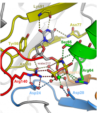
Illustration of the active site of dUTPase from Mycobacterium tuberculosis (PDB ID 1SIX). The orientation of the active site was chosen to feature the geometry of the chemical reaction catalyzed by this enzyme, specifically the in-line nucleophilic attack of water 212 on the alpha-phosphate of dUTP. Fine tuning of the orientation was made to eliminate overlap of side chains and to make all hydrogen bonds (dashed lines) visible. Only side chains directly involved in catalysis are depicted. Carbons are colored according to five conserved motifs of the dUTPase family. Non-conserved residues are given an undistracting gray color and are veiled in fog. Labels were colored to correspond to the side chains they are labeling.

#BEGIN PYMOL SCRIPT for Active Site

set mesh_radius = 0.01 
set antialias = 1 
set stick_radius = 0.22
set dash_radius=0.07
set sphere_scale= 0.22
set ribbon_radius =0.1 
set direct =0.0
set cartoon_fancy_helices=1
bg_color white
set gamma=1.5
util.ray_shadows('none')
set ray_trace_mode=1

# load pdb and map file 
load dumpnpp_10t.pdb, mtb 

cartoon automatic
show cartoon
hide nonbonded
hide lines 

color white, (chain A or chain B or chain C) and (n;ca)
color yellow, (resid 171) or (n;PA) or (n;PB) or (n;PG)
color white, (elem C)
#magnesium
show sphere, (resid 171)
color green, (resid 171)
#waters
show sphere, (resid 173:175 or resid 212)
show sticks, (chain C and resid 170)


color marine, (resid 22:32 and elem C) and chain C
color green, (resid 57:76  and elem C) and chain C
color yellow, (resid 77:93  and elem C) and chain A
color orange, (resid 102:115  and elem C) and chain C
color red, (resid 134:145 and elem C ) and chain B


show sticks, (chain A and resid 83 and  not n;n,c,o )
show sticks, (chain A and resid 86 and  not n;n,c,o )
show sticks, (chain A and resid 77 and  not n;n,c,o )
show sticks, (chain C and resid 24 and  not n;n,c,o)
show sticks, (chain C and resid 28 and not n;n,c,o)
show sticks, (chain B and resid 140 and not n;n,c,o)
show sticks, (chain C and resid 64 and not n;n,c,o)
show sticks, (chain C and resid 113 and not n;n,c,o)
show sticks, (chain C and resid 64:66 )
hide sticks, (chain C and resid 64 and n;n,c,o)
show sticks, (chain A and resid 91 and n;n,c,o,ca)


distance (resid 171 and chain C), (resid 173 and chain C)
color green, dist01
distance (resid 171 and chain C), (resid 174 and chain C)
color green , dist02
distance (resid 171 and chain C), (resid 175 and chain C)
color green , dist03
distance (resid 171 and chain C), (resid 170 and chain C and n;O1A)
color green , dist04
distance (resid 171 and chain C), (resid 170 and chain C and n;O1B)
color green , dist05
distance (resid 171 and chain C), (resid 170 and chain C and n;O1G)
color green , dist06
distance (resid 173 and chain C), (resid 28 and chain C and n;OD2)
color marine, dist07
distance (resid 174 and chain C), (resid 28 and chain C and n;OD1)
color marine, dist08
distance (resid 175 and chain C), (resid 24 and chain C and n;OD2)
color marine, dist09
distance (resid 212 and chain A), (resid 170 and chain C and n;PA)
color red, dist10
distance (resid 212 and chain A), (resid 113 and chain C and n;OE1)
color orange, dist11
distance (resid 212 and chain A), (resid 83 and chain A and n;OD2)
color yellow, dist12
distance (resid 113 and chain C and n;ne2), (resid 170 and chain C and n;O3A)
color orange, dist13
distance (resid 65 and chain C and n;N), (resid 170 and chain C and n;O3A)
color green, dist14
distance (resid 65 and chain C and n;OG), (resid 170 and chain C and n;N2A)
color green, dist15
distance (resid 66 and chain C and n;N), (resid 170 and chain C and n;O3B)
color green, dist16
distance (resid 64 and chain C and n;NH2), (resid 170 and chain C and n;O1B)
color green, dist17
distance (resid 64 and chain C and n;NE), (resid 170 and chain C and n;O1B)
color green, dist18
distance (resid 83 and chain A and n;OD2), (resid 170 and chain C and n;O3')
color yellow, dist19
distance (resid 140 and chain B and n;NH1), (resid 170 and chain C and n;O2G)
color red, dist20
distance (resid 140 and chain B and n;NH2), (resid 170 and chain C and n;O1G)
color red, dist21
distance (resid 140 and chain B and n;NE), (resid 24 and chain C and n;OD1)
color red, dist22
distance (resid 140 and chain B and n;NH2), (resid 24 and chain C and n;OD2)
color red, dist23
distance (resid 170 and chain C and n;O4), (resid 77 and chain A and n;ND2)
color yellow, dist24
distance (resid 170 and chain C and n;N3), (resid 91 and chain A and n;O)
color yellow, dist24
distance (resid 170 and chain C and n;O2), (resid 91 and chain A and n;N)
color yellow, dist24

hide labels

set cartoon_flat_sheets = 1.0
set cartoon_smooth_loops = 0

set_view (\
     0.045321193,    0.677332938,   -0.734195530,\
     0.631984174,   -0.588606596,   -0.504004478,\
    -0.773574233,   -0.441189915,   -0.454773396,\
     0.000917640,    0.000133177,  -65.177696228,\
    14.812702179,    8.131608009,   17.861175537,\
    54.978454590,   79.653022766,    0.000000000 )


# ray 1500,1500
viewport 700,800

Case 3: Structure alignment (≥ novice/intermediate)

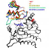
Overlay of aligned alpha-carbon traces

An overlay of five simvastatin synthetase crystal structures illustrating degrees of hinge closing imparted by ligand binding (PDB IDs 3HLB, 3HLC, 3HLE, 3HLF, and 3HLG). Hinge motion in this two-domain enzyme is highlighted by superimposing only atoms in one of the domains (depicted in gray in this figure). The range of motion is highlighted by the rainbow colors assigned to the upper domain. The orientation of the molecule is chosen to make the range of motion evident (hinge axis is normal to the plane of the page). Each of the structures is labeled explicitly in the figure, rather than burying the information in the figure legend. Color coding the labels makes it easier to comprehend how each ligand affects the hinge motion. The structures are represented as a alpha-carbon trace rather than a cartoon ribbon because the motion is relatively small and the alpha carbon trace allows a more exact representation of the position of the atoms.

#BEGIN PYMOL SCRIPT for Overlay of Aligned Molecules

#Load the individual, superimposed molecules
load lovd_c2_refmac10-b_lsq.pdb, G0-Se
load lovd-gx27_refmac11_lsq.pdb, G5
load lovd_gx27-s76a-mja_aps-refmac3_lsq.pdb, G5-S76-MJA
load lovd-gx27-s76a-sim-aps_refmac6_lsq.pdb, G5-S76-Sim
load lovd-gx27-s76a-lov-aps_refmac6.pdb, G5-S76-Lov

hide everything
show ribbon
set ray_trace_mode=0

color red, G0-Se
color orange, G5
color yellow, G5-S76-MJA
color limegreen, G5-S76-Sim
color blue, G5-S76-Lov
color gray, resid 1:92 or resid 204:413

set ribbon_radius=0.3


show sticks, resid 134 and not (name C or name N or name O)
show sticks, resid  86 and not (name C or name N or name O)
show sticks, resn 803
show sticks, G5-MJA and resid 501
show sticks, resid 320  and not (name C or name N or name O) and ( G5-S76-Sim or G5-S76-Lov)
show sticks, resid 334  and not (name C or name N or name O) and ( G5-S76-Sim or G5-S76-Lov)
show spheres, resid 320  and (name od1 or name od2) and G5-S76-Sim
show spheres, resid 334  and (name cg1 or name cg2) and G5-S76-Sim
color red, elem o


set sphere_transparency=0.5
set ray_shadow=off

bg_color white

viewport 1071,1051

set_view (\
     0.836338997,    0.441327691,   -0.325210959,\
     0.390257686,   -0.062672906,    0.918569088,\
     0.385009199,   -0.895153403,   -0.224648848,\
    -0.000003189,    0.000000304, -189.126144409,\
     1.563406944,   17.993612289,  -24.687477112,\
   171.387252808,  203.264083862,    0.000000000 )
~

Case 4: Volumetric data (≥ intermediate)

Electron density map

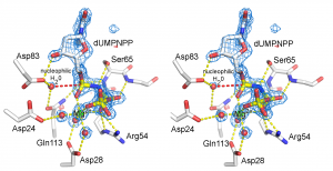
Illustration of an electron density map (omit map) from the enzyme, dUTPase from Mycobacterium tuberulosis (PDB ID 1SIX).

#BEGIN PYMOL SCRIPT Electron Density Map -Left half of stereo image

# general settings
set mesh_radius = 0.015 
set antialias = 1 
set stick_radius = 0.22
set sphere_scale= 0.22
set ribbon_radius =0.1 
# higher values of direct will lighten the image
set direct =0.5
# make the dash lines visible by increasing the thicknes of the dash_radius
set dash_radius = 0.1
#turn of shadows because they complicate the image
util.ray_shadows('none')
bg_color white
 

# load pdb and map file 
load dumpnpp_10t.pdb, mtb 
load omit_twin_out.xplor,  1fofc

# show e-density nearby
# show positive contours of the map 4.2 sigma or higher within 18 angstroms of residue 170 of chain C
isomesh  pos, 1fofc, 4.2, (resid 170 and chain C ), 18.0
color marine, pos
# show negative contours of the map -4.2 sigma or lower within 18 angstroms of residue 170 of chain C
isomesh  neg, 1fofc, -4.2, (resid 170 and chain C ), 18.0
color red, neg
 
cartoon automatic
hide nonbonded
hide lines 

color white, (chain A or chain B or chain C) and (n;ca)
color yellow, (resid 171) or (n;PA) or (n;PB) or (n;PG)
color white, (elem C)
#magnesium
show sphere, (resid 171)
color green, (resid 171)
#waters
show sphere, (resid 173:175 or resid 212)
show sticks, (chain C and resid 170)
show sticks, (chain A and resid 83 and  not n;n,c,o )
show sticks, (chain C and resid 24 and  not n;n,c,o)
show sticks, (chain C and resid 28 and not n;n,c,o)
show sticks, (chain C and resid 64 and not n;n,c,o)
show sticks, (chain C and resid 113 and not n;n,c,o)
show sticks, (chain C and resid 64:66 )

distance (resid 171 and chain C), (resid 173 and chain C)
distance (resid 171 and chain C), (resid 174 and chain C)
distance (resid 171 and chain C), (resid 175 and chain C)
distance (resid 171 and chain C), (resid 170 and chain C and n;O1A)
distance (resid 171 and chain C), (resid 170 and chain C and n;O1B)
distance (resid 171 and chain C), (resid 170 and chain C and n;O1G)
distance (resid 173 and chain C), (resid 28 and chain C and n;OD2)
distance (resid 174 and chain C), (resid 28 and chain C and n;OD1)
distance (resid 175 and chain C), (resid 24 and chain C and n;OD2)
distance (resid 212 and chain A), (resid 170 and chain C and n;PA)
distance (resid 212 and chain A), (resid 113 and chain C and n;OE1)
distance (resid 212 and chain A), (resid 83 and chain A and n;OD2)
distance (resid 113 and chain C and n;ne2), (resid 170 and chain C and n;O3A)
distance (resid 65 and chain C and n;N), (resid 170 and chain C and n;O3A)
distance (resid 65 and chain C and n;OG), (resid 170 and chain C and n;N2A)
distance (resid 66 and chain C and n;N), (resid 170 and chain C and n;O3B)
distance (resid 64 and chain C and n;NH2), (resid 170 and chain C and n;O1B)
distance (resid 64 and chain C and n;NE), (resid 170 and chain C and n;O1B)
distance (resid 83 and chain A and n;OD2), (resid 170 and chain C and n;O3')
color yellow, dist*
color red, dist10

hide labels
 
set_view (\
    -0.350610733,    0.599414885,   -0.719504118,\
    -0.160659447,   -0.795388758,   -0.584337831,\
    -0.922586679,   -0.089291766,    0.375185639,\
     0.002084959,    0.000028796,  -51.327602386,\
    14.307765961,    9.915379524,   17.268175125,\
    42.648197174,   61.923065186,    0.000000000 )
 
turn y, 3.5
viewport 1000, 1000

#ray
#png density-left.png

Case 5: Interfaces (≥ intermediate)

alt text

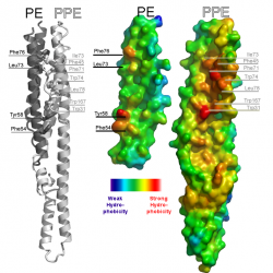
Illustration of an intermolecular interface from the PE-PPE protein complex from Mycobacterium tuberulosis (PDB ID 2G38). The left panel illustrates the complex between PE and PPE proteins as a cartoon ribbon. The two proteins are colored separately to make the interface evident. Hydrophobic side chains involved in the interface are labeled. The right panel illustrates the complementary surfaces of the interface by splitting the complex apart like a clamshell. The smaller protein is the PE protein, the larger protein is the PPE protein. Warm colors indicate strong hydrophobicity; cool colors depict weak hydrophobicity. The left and right panels are depicted on the same scale so the viewer can see how residues labeled on the left correspond to red patches in the surface on the right.

#BEGIN PYMOL SCRIPT -for Intermolecular Interface
#   antialias =1 smooths jagged edges, 0 turns it off
set antialias = 1
set direct =0.3
set transparency=0.0
set ray_trace_mode=0
set sphere_transparency=0.0
set light_count=2
set ray_shadow=on
set ray_shadows=on
set orthoscopic = on
set opaque_background,0
# control the position of the light so shadows are cast
# in cavities of  the molecular surface
set light =[ -0.50000, -0.70000, -0.750000 ]


#   stick_radius -adjust thickness of atomic bonds
set stick_radius = 0.8
set line_radius = 0.01
set sphere_scale = 0.35
set cartoon_rect_width=0.5
set cartoon_rect_length=2.2
set cartoon_loop_radius=0.4

#   bg_color --set the background color
bg_color white

#   load pdb file and give it an object name
load pe-trans-hydrofob.pdb, pe
load ppe-trans-hydrofob.pdb, ppe
load pe-rot-hydrofob.pdb, pe-hydrofob
load ppe-rot-hydrofob.pdb, ppe-hydrofob

#   show cartoon ribbons
show cartoon, pe or ppe
show surface, pe-hydrofob or ppe-hydrofob

#   hide nonbonded atoms (i.e. waters)
hide nonbonded


#   Hide the default line representation of atomic bonds
hide lines

#   Use standard helix, strand, and loop representations
#   other possibilities: cartoon loop, cartoon rect,
#   cartoon oval, and cartoon tube
cartoon automatic

#   If you dont have secondary structure assignments
#   in the PDB header then uncomment the following
#   line to detect secondary structure.
#   util.ss 1a2w
#   Warning, very coarse approximation.
#   Or get secondary structure assignments from dssp
#   http://swift.cmbi.kun.nl/gv/dssp/
#   Then convert assignments into a PDB header
#   http://structure.usc.edu/dssp2pdb/
#If you want to define secondary structure manually, 
#Use the following syntax
#alter B/753:758/, ss='S'



#   Make fancy helices with ridge on the edges like
#   molscript does
#   1 is on.  0 is off.
set cartoon_fancy_helices=1

#   Make the strands flat=1 or pass through CA positions=0
#   Set to 0 when showing side chains from a strand
set cartoon_flat_sheets = 1.0

#   Draw the loops smooth=1 or pass through CA positions=0
#   Set to 0 when showing side chains from a loop
set cartoon_smooth_loops = 0

#   Set the color of the residues
#   to find the names of the colors available
#   click on the rainbow colored square in the
#   upper right corner of the graphics window


# hydrophobicity values are printed in the B-factor column
# of the pdb file. So, color by  B-factor.
cmd.spectrum("b",selection=("pe-hydrofob"),quiet=0)
cmd.spectrum("b",selection=("ppe-hydrofob"),quiet=0)
cmd.spectrum("b",selection=("pe"),quiet=0)
cmd.spectrum("b",selection=("ppe"),quiet=0)

color white, ppe 
color gray, pe 

#   Show spheres for cysteine sulfurs
show spheres, name sg 

#   Show sticks for bonds
show sticks, (resn cys) and not (name n,c,o)

show sticks, chain B and (resid 31 or resid 167 or resid 74 or resid 78 or resid 71 or resid 45 or resid 173) and not (name n or name c or name o)
show sticks, chain A and (resid 58 or resid  54 or resid 76 or resid 73) and not (name n or name c or name o)

hide labels

set_view (\
    -0.881387651,   -0.417317063,    0.221362144,\
     0.171217963,    0.154523358,    0.973037899,\
    -0.440271527,    0.895526111,   -0.064742655,\
     0.000100300,   -0.000183796, -328.588287354,\
     4.581910610,   13.162490845,   90.285400391,\
   270.283447266,  386.892944336,    1.000000000 )


viewport 600, 700

Case 6: Higher-order structures (≥ intermediate/advanced)

Case 7: Animations (≥ intermediate/advanced)

See the Animations section below.

Case 8: Best-fit planes (≥ advanced)

Animations

A classification scheme

The possible types of 3D figures and animations are enumerated in Table 1. Below the symbol for each category is a tangible example of that particular type of illustration. The principles and practices used to create superb static figures (i.e., M_sV_s) also apply to the design and rendering of animations, each frame of which can be essentially considered a stand-alone figure.

**Table 1**: A classification of figures & animations.
		Coordinates of molecular entities ('M')
		static	dynamic
Viewpoint ('V')	static	M_sV_s A standard (static) molecular illustration	M_dV_s Visualize an MD trajectory from a single/fixed viewpoint
Viewpoint ('V')	dynamic	M_sV_d A rotating camera 'scan' of the molecular objects	M_dV_d Visualize a trajectory from dynamically changing viewpoints

M_sV_s — Molecule is static, View is static

These are simply the 'ordinary', static figures illustrated by most of the case studies in this tutorial.

M_sV_d — Molecule is static, View is dynamic

M_dV_s — Molecule is dynamic, View is static

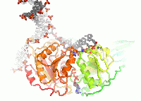
Movie of a DNA helicase unwinding dsDNA (animated GIF format)

A movie illustrating conformational changes in a helicase as it unwinds double stranded DNA.

#BEGIN PYMOL SCRIPT
#   antialias =1 smooths jagged edges, 0 turns it off
set antialias = 1
set ambient = 0.3
set light_count = 6

#   stick_radius -adjust thickness of atomic bonds
set stick_radius = 0.6
set sphere_scale = 0.5
set cartoon_rect_width=0.9
set cartoon_rect_length=2.0
set cartoon_loop_radius=0.5
#   mesh_radius -to adjust thickness of electron
#   density contours
set mesh_radius = 0.02

#   bg_color --set the background color
bg_color white

#   load pdb file and give it an object name
load ff01.pdb,mov,1
load ff02.pdb,mov,2
load ff03.pdb,mov,3
load ff04.pdb,mov,4
load ff05.pdb,mov,5
load ff06.pdb,mov,6
load ff07.pdb,mov,7
load ff08.pdb,mov,8
load ff09.pdb,mov,9
load ff10.pdb,mov,10
load ff11.pdb,mov,11
load ff12.pdb,mov,12
load ff13.pdb,mov,13
load ff14.pdb,mov,14
load ff15.pdb,mov,15
load ff16.pdb,mov,16
load ff17.pdb,mov,17
load ff18.pdb,mov,18
load ff19.pdb,mov,19
load ff20.pdb,mov,20
load ff21.pdb,mov,21
load ff22.pdb,mov,22
load ff23.pdb,mov,23
load ff24.pdb,mov,24
load ff25.pdb,mov,25
load ff26.pdb,mov,26
load ff27.pdb,mov,27
load ff28.pdb,mov,28
load ff29.pdb,mov,29
load ff30.pdb,mov,30



#   hide nonbonded atoms (i.e. waters)
hide nonbonded

#   show cartoon ribbons
show cartoon, chain a

#   Hide the default line representation of atomic bonds
hide lines

#   Use standard helix, strand, and loop representations
#   other possibilities: cartoon loop, cartoon rect,
#   cartoon oval, and cartoon tube
cartoon automatic

#   If you dont have secondary structure assignments
#   in the PDB header then uncomment the following
#   line to detect secondary structure.
#   Warning, very coarse approximation.
#   Or get header from http://www.mbfys.lu.se/Services/SecStr/
#util.ss 1a2w

#   Make fancy helices with ridge on the edges like
#   molscript does
#   1 is on.  0 is off.
set cartoon_fancy_helices=1

#   Make the strands flat=1 or pass through CA positions=0
#   Set to 0 when showing side chains from a strand
set cartoon_flat_sheets = 1.0

#   Draw the loops smooth=1 or pass through CA positions=0
#   Set to 0 when showing side chains from a loop
set cartoon_smooth_loops = 0

#   Set the color of the residues
#   to find the names of the colors available
#   click on the rainbow colored square in the
#   upper right corner of the graphics window
util.chainbow("(mov)")

#   Show spheres for chloride ions
#show spheres, name sg 

#   Show sticks for bonds
#show sticks, (resn cys) and not (name n,c,o)
show sticks, resn atp or resn po4
show sticks,  resn adp or chain e or chain d
show sticks, (resid 540 or resid 563 or resid 545 or resid 377 or resid 358 or resid 335 or resid 373 or resid 475 or resid 483 or resid 485) and not (name c or name o or name n)
hide cartoon, chain e or chain d or resn atp or resn adp or resn po4

color red, elem o
color blue, elem n
color gray,  chain d
color white, chain e
color orange, elem p
color gray, elem c and (resn po4 or resn adp or resn atp)
color firebrick, elem o and (name o1p or name o2p or name o3' or name o5')
unbond resn po4, resn adp

#alter B/753:758/, ss='S'

# set up simple rotation commands

mset 1 - 15

### cut below here and paste into script ###
set_view (\
     0.017624758,   -0.997306943,   -0.071203344,\
    -0.656398058,    0.042179316,   -0.753232718,\
     0.754207492,    0.060014214,   -0.653885424,\
     0.000000950,   -0.000033716, -206.950531006,\
    45.939758301,   43.484542847,   46.991050720,\
   159.799530029,  216.515686035,    0.000000000 )
### cut above here and paste into script ###



#set ray_trace_mode=3
viewport 700,500

#### make output directory (NOTE: preceeding "/" = literal python)

/if not os.path.exists("png"): os.mkdir("png")

####enable raytracing

set ray_trace_frames=1
set cache_frame=0

#### render

mpng png/mov

M_dV_d — Molecule is dynamic, View is dynamic

Useful links

A compilation of links and other online resources that were helpful in creating these examples. Please edit as you see fit.

PyMOL-related

PyMOL's list of links to user-maintained script collections, tutorials, etc. - http://pymol.org/links.html

Python-related

General MolVis

Conceptual background
- Useful general info (historical & conceptual), links, etc. - http://en.wikipedia.org/wiki/Molecular_graphics
- The "graphics pipeline" - http://en.wikipedia.org/wiki/Graphics_pipeline

Historical background & significance
- Martz & Francoeur's online history of MolVis - http://www.umass.edu/microbio/rasmol/history.htm
- Levinthal's account of the early days -

Individual pages, script repositories, etc.
- Lev Gelb's (WashU) MolVis page - http://www.chemistry.wustl.edu/~gelb/visualization.html

Abbreviations, symbols, etc.

The following abbreviations, acronyms, or other symbols may be encountered on this wiki page:

"dsDNA" = double-stranded DNA
"API" = Application Programming Interface

@@ Line 537: / Line 537: @@
 == <span style="font-weight:normal;">A classification scheme</span> ==
-The possible types of 3D figures and animations are enumerated in Table 1. Below the symbol for each category is a tangible example of that particular type of illustration. The principles and practices used to create superb static figures (M<sub>s</sub>V<sub>s</sub>) also apply to the design and rendering of animations, each frame of which can be essentially considered a stand-alone figure.
+The possible types of 3D figures and animations are enumerated in Table 1. Below the symbol for each category is a tangible example of that particular type of illustration. The principles and practices used to create superb static figures (''i.e.'', M<sub>s</sub>V<sub>s</sub>) also apply to the design and rendering of animations, each frame of which can be essentially considered a stand-alone figure.
 {|border="0" style="width:40%; border-collapse:collapse;"

PLoS: Difference between revisions

Revision as of 23:29, 2 January 2010

Contents

Overview, general notes

Figures

Case 1: Overall fold / domain level (≥ novice/intermediate)

Case 2: Ligand-binding sites (≥ novice/intermediate)

Case 3: Structure alignment (≥ novice/intermediate)

Case 4: Volumetric data (≥ intermediate)

Case 5: Interfaces (≥ intermediate)

Case 6: Higher-order structures (≥ intermediate/advanced)

Case 7: Animations (≥ intermediate/advanced)

Case 8: Best-fit planes (≥ advanced)

Animations

A classification scheme

M_sV_s — Molecule is static, View is static

M_sV_d — Molecule is static, View is dynamic

M_dV_s — Molecule is dynamic, View is static

M_dV_d — Molecule is dynamic, View is dynamic

Useful links

PyMOL-related

Python-related

General MolVis

Abbreviations, symbols, etc.

Navigation menu

PLoS: Difference between revisions

Revision as of 23:29, 2 January 2010

Overview, general notes

Figures

Case 1: Overall fold / domain level (≥ novice/intermediate)

Case 2: Ligand-binding sites (≥ novice/intermediate)

Case 3: Structure alignment (≥ novice/intermediate)

Case 4: Volumetric data (≥ intermediate)

Case 5: Interfaces (≥ intermediate)

Case 6: Higher-order structures (≥ intermediate/advanced)

Case 7: Animations (≥ intermediate/advanced)

Case 8: Best-fit planes (≥ advanced)

Animations

A classification scheme

MsVs — Molecule is static, View is static

MsVd — Molecule is static, View is dynamic

MdVs — Molecule is dynamic, View is static

MdVd — Molecule is dynamic, View is dynamic

Useful links

PyMOL-related

Python-related

General MolVis

Abbreviations, symbols, etc.

Navigation menu

Search

M_sV_s — Molecule is static, View is static

M_sV_d — Molecule is static, View is dynamic

M_dV_s — Molecule is dynamic, View is static

M_dV_d — Molecule is dynamic, View is dynamic